This project, conducted as part my Data Science for Business course at Aalto University, focuses on building a predictive lead scoring model for X Education, an online course provider for industry professionals. The company faces a low lead-to-customer conversion rate of 30% and aims to increase this to 80% by identifying and prioritizing “Hot Leads” — prospects most likely to convert into paying customers.
The model uses historical lead data from Kaggle, applies rigorous data preprocessing, and evaluates multiple machine learning algorithms, including Logistic Regression, Decision Tree, Support Vector Machine, and XGBoost.
Key finding:
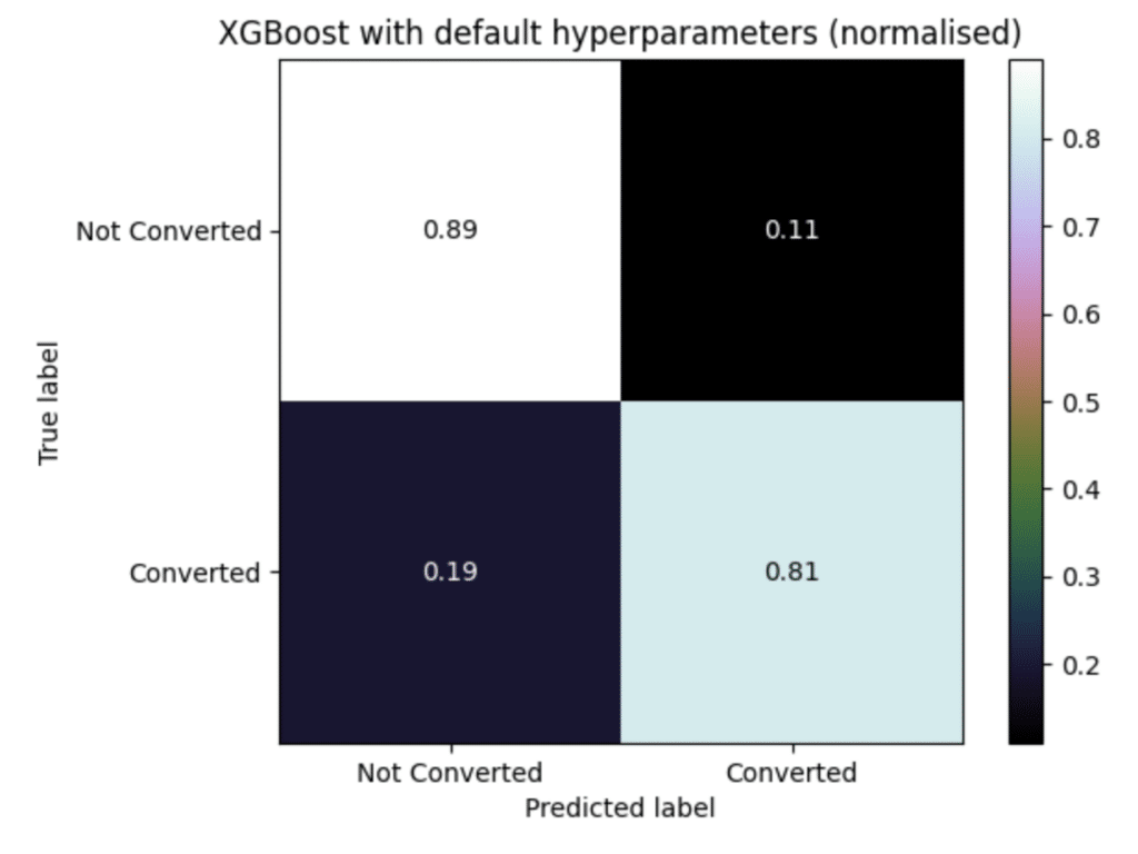
The XGBoost model with default hyperparameters achieved the best results (accuracy 0.8578, TPR 0.81), making it the most suitable choice for deployment. Feature importance analysis provided actionable insights for marketing and sales strategies, such as targeting working professionals and housewives, and reassessing digital ad performance.


Steps to Build the Predictive Model
- Define the Problem and Objective: Clearly articulate the business objective—to increase the lead conversion rate to 80% by identifying the most promising leads.
- Explore and Preprocess Data: Analyze the raw dataset to understand its structure. Clean the data by removing irrelevant columns, handling missing values, and transforming categorical and numerical features for modeling.
- Build and Select Models: Split the data into training and testing sets. Implement and compare various classification algorithms (e.g., Logistic Regression, Decision Tree, XGBoost).
- Evaluate the Models: Use key performance metrics like accuracy, F1-Score, and the True Positive Rate from confusion matrices to assess and compare model performance. Select the model that best aligns with the business goal.
- Interpret Results and Apply: Use the chosen model to score leads. Extract insights from important features to inform business strategy and provide actionable recommendations for sales and marketing teams.
Define the Problem and Objective
In this project, we used a dataset available in Kaggle.
About the Dataset
An education company named X Education sells online courses to industry professionals. On any given day, many professionals who are interested in the courses land on their website and browse for courses.
The company markets its courses on several websites and search engines like Google. Once these people land on the website, they might browse the courses or fill up a form for the course or watch some videos. When these people fill up a form providing their email address or phone number, they are classified to be a lead. Moreover, the company also gets leads through past referrals. Once these leads are acquired, employees from the sales team start making calls, writing emails, etc. Through this process, some of the leads get converted while most do not. The typical lead conversion rate at X education is around 30%.
Now, although X Education gets a lot of leads, its lead conversion rate is very poor. For example, if, say, they acquire 100 leads in a day, only about 30 of them are converted. To make this process more efficient, the company wishes to identify the most potential leads, also known as ‘Hot Leads’. If they successfully identify this set of leads, the lead conversion rate should go up as the sales team will now be focusing more on communicating with the potential leads rather than making calls to everyone.
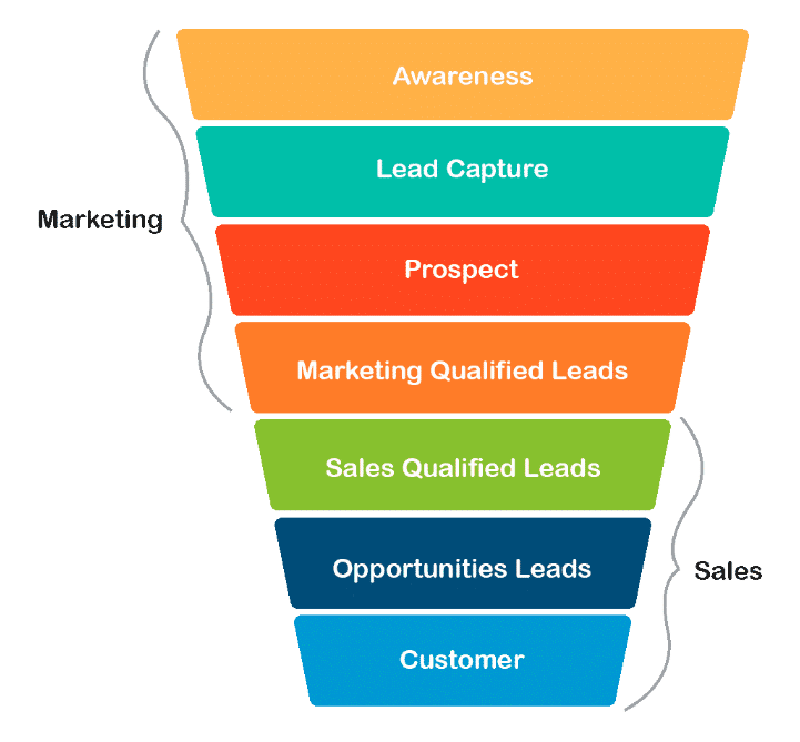
There are a lot of leads generated in the initial stage (top) but only a few of them come out as paying customers from the bottom. In the middle stage, you need to nurture the potential leads well (i.e. educating the leads about the product, constantly communicating, etc. ) in order to get a higher lead conversion.
X Education wants to select the most promising leads, i.e. the leads that are most likely to convert into paying customers. The company requires you to build a model wherein you need to assign a lead score to each of the leads such that the customers with higher lead score h have a higher conversion chance and the customers with lower lead score have a lower conversion chance. The CEO, in particular, has given a ballpark of the target lead conversion rate to be around 80%.
Business problem and motivation
Central to the business problem is the concept of “Lead Scoring.” Lead Scoring involves assigning a numerical score to each lead, representing their likelihood of converting into a paying customer. This score is calculated using various lead attributes and behaviors.
The study of this problem is beneficial to multiple stakeholders. Early detection of potential leads enables timely and tailored interactions, consequently improving conversion rates. Focused resource allocation enhances sales and marketing team efficiency, reducing wastage on low-quality leads. This efficiency enhances sales productivity as representatives prioritize high-quality leads, increasing success rates. Moreover, by uncovering influential conversion variables, this project empowers data-driven decision-making, optimizing marketing and sales strategies for more effective campaigns and customer interactions. The insights will have broader applicability across businesses facing similar lead management challenges.
Aims of the study
The objective of this study is to create a classification model that assigns a score to each lead and assists the business goal of achieving 80% conversion rate.
The goal is to filter out lower-quality leads and concentrate resources on nurturing the most promising ones through the lead scores as the results of the selected model.
Exploring and Preprocessing Data
Explore the data
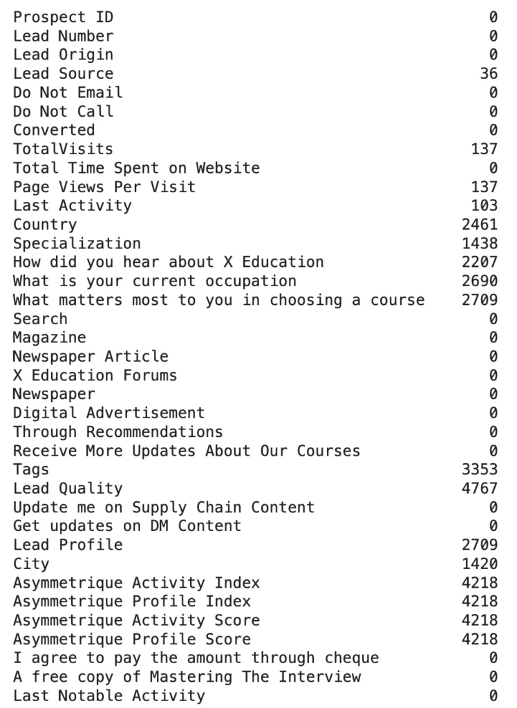
The raw dataset contains 9240 rows and 37 variables, including target variable.
There are 30 categorical variables and 7 numerical variables. 17 variables have missing values.
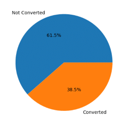
The target variable is Converted, indicating whether a lead has been successfully converted or not. From the original dataset, 61.5% of leads have not converted and 38.5% of leads have successfully converted into customers.
Preprocessing the data
Removing variables
- Drop Prospect ID and Lead Number since they are identification numbers.
- Drop columns that contain only one unique value such as Magazine, Receive More Updates About Our Courses, Update me on Supply Chain Content, Get updates on DM Content, I agree to pay the amount through cheque.
- Drop columns that are redundant (How did you hear about X Education, Tags, What matters most to you in choosing a course), have little impact on the problem (Do Not Email, Do Not Call, A free copy of Mastering The Interview), and the columns that contain information influenced by internal employees as such data may introduce bias and not reflect the full scope of lead characteristics (Lead Quality, Lead Profile). We also drop Country column since this company primarily operates within India.
Handling missing values
- For the numerical variables: filling in missing values with the mean value of the respective feature.
- For the categorical variables: replacing missing values with a new Undefined category.
Transforming data
- Converting variables with Yes/No values to 1/0.
- Converting features with values that have an ordinal relationship High/Medium/Low/Undefined to 3/2/1/0.
- For categorical features, grouping values with less frequency into Others group.
- Using one-hot encoding to convert the categorical variables.
- After data manipulation, the dataset contains 9240 rows and 88 variables.
Building the Model
After data transformation, we split the dataset into training (70%) and testing (30%) partitions for model building and evaluating.
We applied several methods to compare their performance and selected the most appropriate model for our business case.
- Logistic regression
- Decision tree
- Support vector machine
- Ensemble method (XGBoost)
We also optimised the model performance by trying different hyperparameter tuning methods and conducting feature selection.
Decision Tree
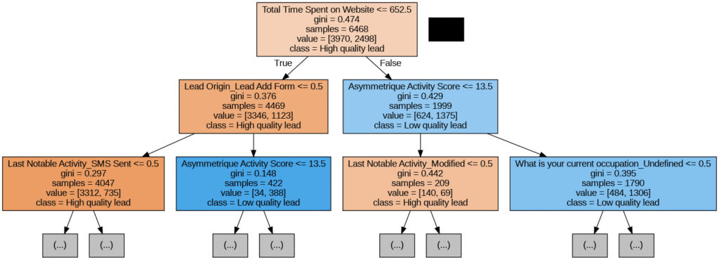
Implementing a decision tree was a very effective way to visualize how the variables of our dataset can help us distinguish high from low quality leads. Experimenting with different levels of depth in order to find the best performing, we ended up selecting a tree with 5 levels of depth and 29 nodes, which is not fully represented in the image above due to its huge dimensionality. This decision tree already had a high accuracy value, above 0.83, which led us to deduct that the variables of our dataset were quite successful when discerning the outcome and that we could build a model with an even higher predictive power.
Logistic Regression
Another method that we used to approach our business problem was logistic regression. Logistic regression was chosen because we worked with a classification problem, and with logistic regression one can interpret the probability that the label of x is 1.¹ That is, it is possible to find out the probability of a lead converting to a customer.
First, we computed a default logistic regression that we could use as a baseline later. Then we proceeded to improve our logistic regression model.
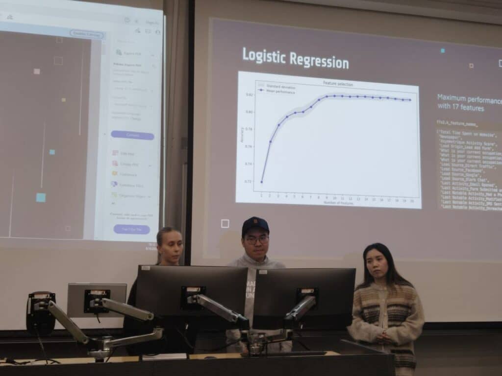
Feature selection
The first step of improving our model was feature selection. As our data set is large, we chose to use forward selection and set the maximum number of features to 25. If the model performance would improve even after adding the 25th feature, we would re-run the feature selection with a higher maximum number of features. In the feature selection phase, we also set scoring to “accuracy” and used cross-validation.
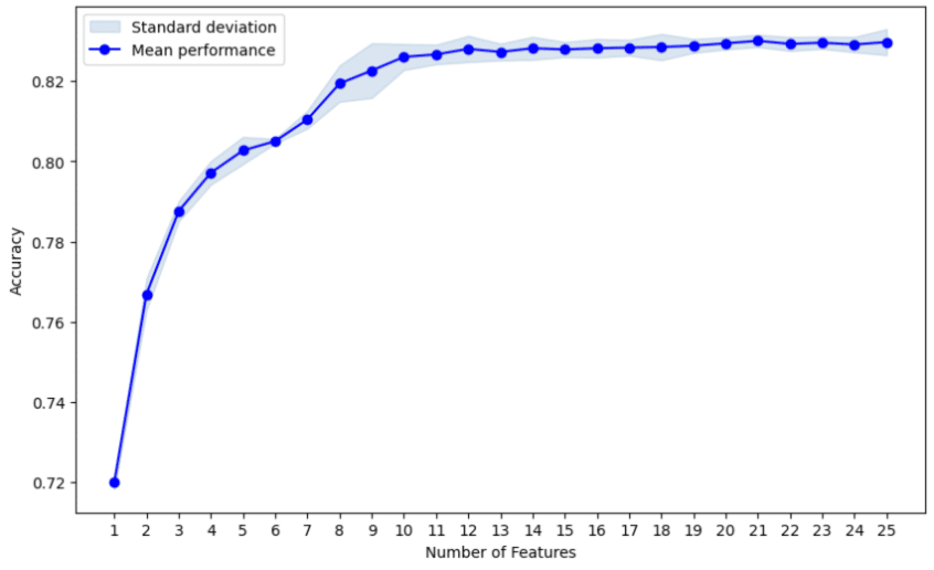
From the figure we can see that the accuracy stops improving quite quickly. From feature names, on the next page, we can see that the maximum performance is reached with 21 features. Therefore, there was no need to re-run forward selection with higher number of features.
Feature selection – results
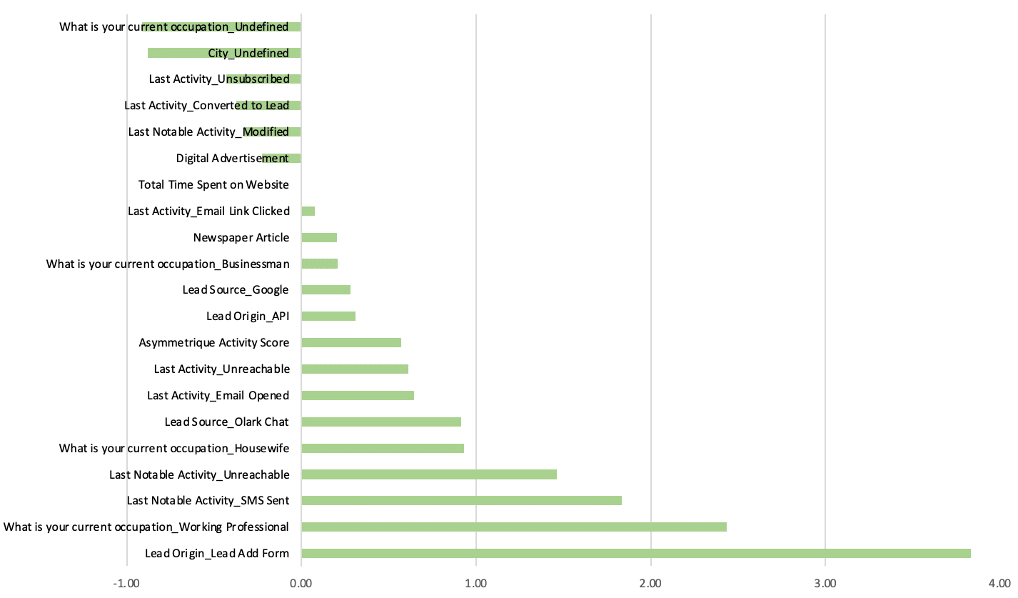
The figure shows us the 21 selected features. The biggest negative effect came from undefined occupation and undefined city. That is, people who do not provide this kind of information about themselves seem to be less interested in the company’s products.
The biggest positive effect came from lead add form as a lead origin – the origin identifier with which the customer was identified to be a lead. The second biggest effect came from working professional as an occupation.
Our feature selection model reached the accuracy of 0.82, while our baseline logistic regression had the accuracy of 0.82 as well. This indicates that feature selection did not manage to improve our model’s performance, at least based on accuracy.
Hyperparameter tuning
As our aim was to improve our model’s performance, we moved on to hyperparameter optimisation. We used GridSearchCV from Python’s scikit-learn package for hyperparameter optimisation. We optimised the following parameters: penalty, C (regularisation strength) and max_iter. We set scoring to “accuracy”. For regularisation strength we got a value of approximately 0.62, maximum number of iterations was set to 5000 and for penalty we got l2. The accuracy of our model after the hyperparameter tuning was 0.84. That is, we managed to get a slightly better accuracy, even though the difference is not big.
Logistic regression model evaluation
After conducting a default logistic regression and performing feature selection and hyperparameter optimisation, we evaluated these models based on different criteria. This was done to gain better understanding of the performance of our models and to determine which model performs the best. In addition to accuracy, we looked at confusion matrices and receiver operating characteristic curves (ROC curves). From confusion matrices we got true positive rate, true negative rate, precision and F1 score. From ROC curves we also got the area under curve (AUC) value.
| Default logistic regression | Feature selected logistic regression | Hyperparameter tuned logistic regression | |
| Accuracy | 0.82 | 0.82 | 0.84 |
| True positive rate | 0.74 | 0.73 | 0.76 |
| True negative rate | 0.87 | 0.88 | 0.89 |
| Precision | 0.78 | 0.79 | 0.81 |
| F1-Score | 0.76 | 0.76 | 0.78 |
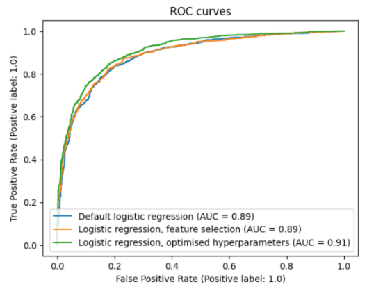
From the table and figure above, we see that the default logistic regression model performed nearly as well as the feature selected model. The true positive rate of the default model is higher, otherwise the feature selected model is slightly better or just as good. Although the differences are not big, the hyperparameter tuned logistic regression model performs best in our evaluation. The values from confusion matrix are better, as is the AUC value. Thus, we can conclude that it’s the best of these three logistic regression models.
Bayesian Optimisation
Using Support Vector Classification as the estimator, we developed another model using optimised hyperparameters. However, this model did not perform better than the one built using Grid Search.
XGBoost
Finally, we used ensemble methods to create a stronger model. We applied extreme gradient boosting with both default and optimised hyperparameters. Unsurprisingly, they outperformed all the previous models. The model with Optuna search optimisation had a particular high score of above 0.85.
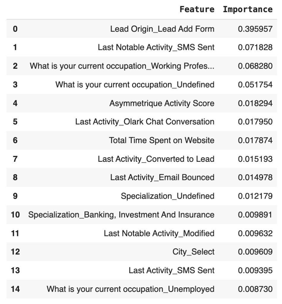
We can see a table presenting the 15 most important features for the XGBoost model with default hyperparameters. This group of highlighted features is very similar to the one selected by our logistic regression model. It is noteworthy to pinpoint that lead add form as a lead origin was again the feature with the highest importance value. In this model, its significance is even higher in comparison to the other selected features.
Model Evaluation
| Hyperparameter tuned logistic regression | Decision tree | Bayesian optimisation with SVM | XGBoost with default hyperparameters | XGBoost with Optuna search optimisation | |
| Accuracy | 0.8395 | 0.8348 | 0.8359 | 0.8578 | 0.8571 |
| Precision | 0.8121 | 0.8174 | 0.7929 | 0.8201 | 0.8241 |
| F1-Score | 0.7832 | 0.7728 | 0.7834 | 0.8131 | 0.8107 |
On the above table, we can analyse how the best logistic regression model performs in comparison to the decision tree, bayesian optimisation and XGBoost models, in terms of accuracy, precision and F1-score. While it outperforms the first two models, the hyperparameter tuned logistic regression is still weaker than the ensemble models.
Against our previous findings, the XGBoost model with default hyperparameters has a slightly higher accuracy value than the optimised one. Its F1-Score is also the highest, while the optimised gradient boosting model has the best precision outcome. Since the difference between these models is basically residual, it is best for X Education to adopt the simplest one.
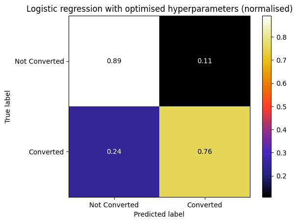
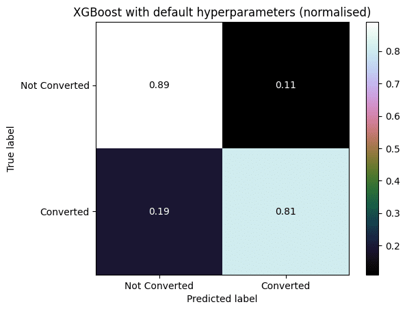
The comparison between these two confusion matrices is a good example of how the XGBoost models outperform all the others. As we can see, the logistic regression model with optimised hyperparameters and the default XGBoost model have the same True Negative Rate (0.89). However, the True Positive Rate model for the first model is only 0.76, while for the latter it is 0.81. This discrepancy is a constant between the XGBoost models and the other ones. This is vital for our business problem, since it is very important for X Education’s sales team not to waste time with low quality leads (False Positive cases), in order to optimise time management and increase sales.
ROC and AUC
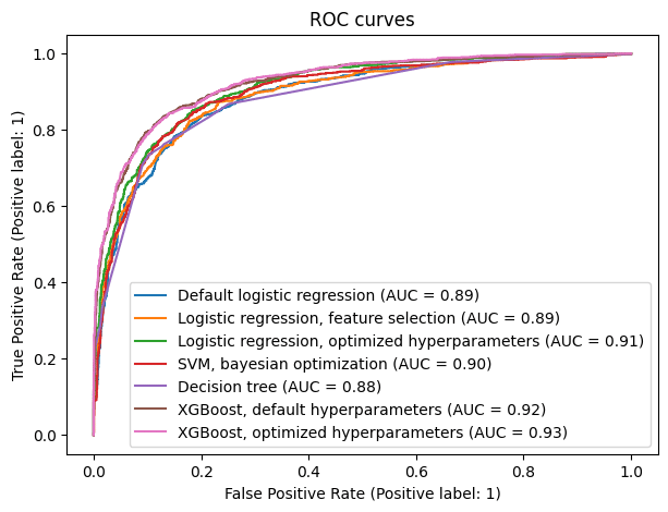
As we did previously with our logistic regression models, now we see the ROC curves for all predictive models, so that we can have a visual interpretation of their sensitivity-specificity trade off.
Once again, the ensemble models display the best results, exceeding all the other ones in each point of the graph. Therefore, independently of the objectives set by X Education, it is correct to adopt any of the XGBoost models.
Despite the extreme gradient boosting model with optimised hyperparameters having a higher AUC (0.93) than its counterpart (0.92), the difference is not significant, so we still keep the simplest model.
Results
All the models are quite good at finding True Positives (Converted) and True Negatives (Not Converted). However, as we are looking for high-quality leads with the high possibility of converting into paying customers, the XGBoost with default hyperparameters is the most suitable model. The extreme gradient boosting model with default hyperparameters not only has the highest accuracy than its counterpart (0.8578), but it is also the model that can predict True Positives best (81%).
The results from feature selected logistic regression model as well as the XGBoost model revealed that some variables have a stronger impact in our models than others. This kind of information is valuable for conducting future marketing strategies and budget. For example, working professionals and housewives had a positive impact on conversion and therefore the company should target individuals with these occupations in its advertising. On the contrary, we can see what kind of individuals are not as potential customers. We also saw that in the feature selected logistic regression model “Digital advertisement” had a negative impact, which indicates that the company’s digital advertising has not brought high-quality leads and therefore should be improved or that digital advertisements should not be prioritised in the company’s advertising strategy.
Conclusions and Applications
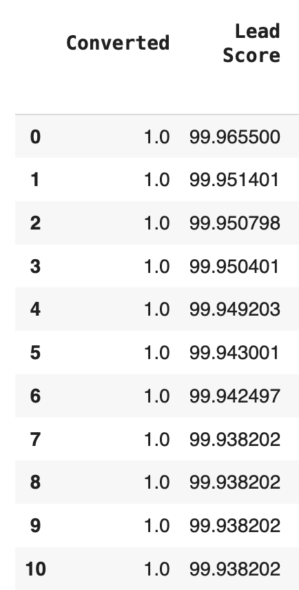
The probability of each lead as the results of the model will be used as lead score.
Lead score will help Sales team prioritize and focus their effort on leads with higher scores, improving the overall efficiency of the lead conversion process.
The model will provide a consistent and objective way to assess lead quality, hence, the company will transition from a more intuitive lead conversion process to a data-driven approach.
Suggestions for further study Refinement of Features:
- Refinement of Features: Dive deeper into feature importance/feature selection to find out characteristics of hot leads and which marketing activities bring more high quality leads. Are there additional features or data sources that can be incorporated into the lead scoring model to improve its accuracy and predictive power?
- Model Evaluation: The lead scoring model can be continually improved by analyzing conversion outcomes. Are the predicted lead scores aligning with actual conversion rates? What is the impact on the overall conversion rate?
- Lead Nurturing Strategies: How can we tailor lead nurturing strategies based on lead scores? What kind of marketing channels and content are most effective for different lead segments?